EBWM: Cognitively Inspired Energy-Based World Models
Paper: https://arxiv.org/abs/2406.08862
TLDR:
We developed a new approach for Autoregressive (AR)/world modeling1 called Energy-Based World Models (EBWM).

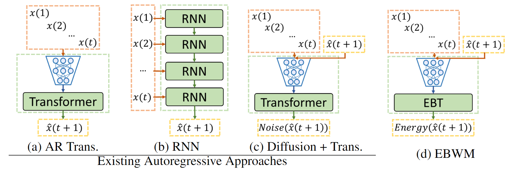
This is inspired by several facets of human cognition, such as System 2 thinking from psychology (which is prolonged, deliberate, and dynamic thinking). Existing AR approaches cannot achieve all cognitive facets discussed in the paper while EBWM can.
EBWM scaled better than traditional autoregressive transformers in data efficiency and GPU hours at sequence modeling in CV.
This blog is written for readers not familiar with all topics discussed, and therefore makes simplifications when describing various topics. Feel free to skip certain sections that are review for you.
Problems with Current Models
Large Language Models (LLMs) have achieved amazing feats, but still struggle to reason and plan. So how can we train LLMs, and more broadly, world models to reason and plan like humans? Our new work, Cognitively Inspired Energy-Based World Models, aims to address this.
To understand why current LLMs/world models cannot reason and plan at the level of humans, consider the two questions below:
What is 2 + 2?
What is 67 * 54?
These questions vary drastically in difficulty—the first you could probably solve without even deliberately thinking but the second would take deliberate mathematical reasoning. Yet, most existing world models are trained to make every prediction with a fixed amount of computational resources (If you’re thinking CoT is a counterexample to this check the paper!) As humans, we naturally adjust the computational resources we use towards the difficulty of the problem, which is more broadly referred to as System 2 thinking in psychology.
We trained world models to be able to approximate aspects of System 2 thinking, through developing ‘Energy-Based World Models’ (EBWM). Not only are these models able to dynamically allocate compute based on the difficulty of a given problem during inference, but they can also achieve several other facets of cognition not possible with existing traditional autoregressive approaches (e.g. Autoregressive Transformers, RNNs, Diffusion Transformers, etc).
This matters, because it provides promising steps towards training world models that can truly think, reason, and plan, at the same level as humans—a problem I’m confident is one of the largest blockers towards achieving human-level intelligence/AGI.
Before we continue, let’s review what some of the topics we’ll be discussing are.
Review
World Models
Intuitively, world models are predictive models of the world. They have learned various laws of physics, such as gravity, and know how people move, how the sun sets, and various other aspects of the world. The world models that our paper focused on are a specific instance of world models where there are several sensory inputs (i.e. multiple video frames) and the model is trained to predict the next sensory input (i.e. the next frame)2. Mathematically, this is equivalent to the following:
\[x(t+1) = F(x(1), x(2), \ldots, x(t))\]Where $x(1), …, x(t+1)$ are sensory inputs (i.e. different video frames) and F is the function (or more specifically energy function) being learned.
Energy-Based Models
Energy-Based Models (EBMs) assign a scalar value, called the energy, to each configuration of inputs to a model. The key idea is that configurations with lower energy are more probable and compatible with each other, while those with higher energy are less likely. The goal of an EBM is to learn an energy function (which is usually just a neural network/the model) that gives lower energy to “correct” or “desirable” configurations, like real data points, and higher energy to “incorrect” or “undesirable” ones, like noise or outliers.
In the context of world models trained as EBMs, you can think of this energy as how probable/compatible the predicted next state is with the context/past.
For example, if the given context was a video of a red ball flying up through the air, a high energy continuation may be a video of a dog chewing on its toy, while a low energy continuation might be a red ball flying down through the air. This red ball flying down through the air is more compatible with the context, which implies lower energy.
Markov Chain Monte Carlo
EBMs trained with neural networks (NNs) have some cool characteristics. Since NNs are fully differentiable, these models can use a method called Markov Chain Monte Carlo (MCMC). Simply put, MCMC under the context of EBMs is a technique that helps models start from random noise and iteratively improve upon their predictions. It does this by minimizing the learned energy function, or by backpropagating the gradient from the energy scalar to the input being improved upon. You can think about this intuitively as asking the model, “How can I adjust this input to improve its likeliness”, and the model telling you how to adjust each and every aspect of the input (i.e. each pixel in the video frame) to minimize the energy and therefore increase that input’s compatibility with the other inputs.
EBWM
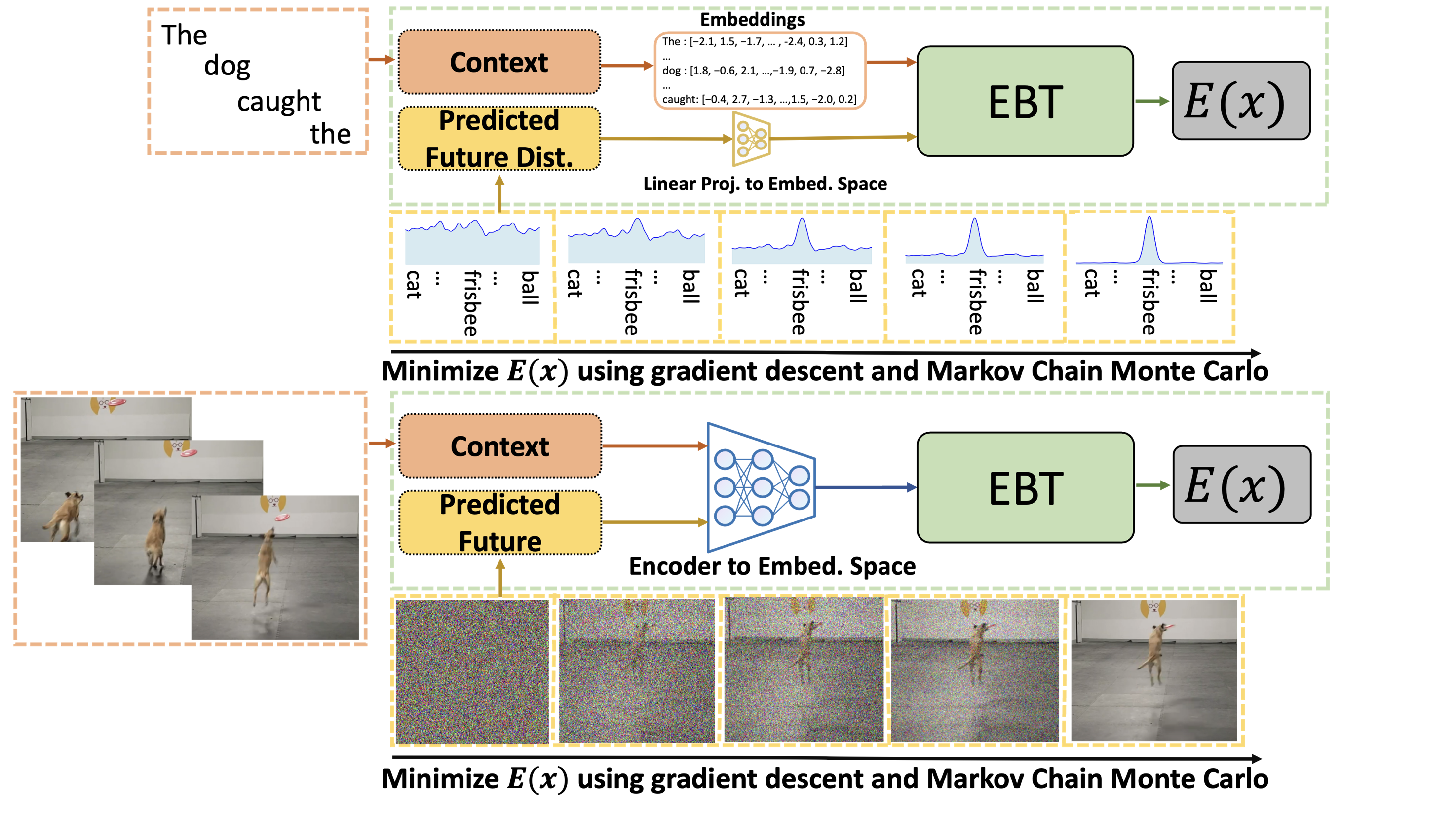
Now, let’s take a look at EBWM in NLP and CV (note that we visualize words and images for NLP and CV respectively, but note that this is all done at the token/embedding level):

The orange boxes here represent the context. The yellow boxes represent the predicted future state (which starts as random noise). First, EBWM predicts the energy of the initially predicted future state (which is likely to be high since it is random noise). Then, using MCMC, this prediction is iteratively improved upon. This ability to dynamically improve upon predictions, while giving an energy score for each of them, allows the models to achieve several cognitive feats described below.
Energy-Based Transformer
The Energy-Based Transformer can just be thought of as a decoder transformer with causal attention specifically made to be parallelizable for EBMs. To understand why this is necessary, please check the paper.
Implementation Details
The pseudocode is really helpful for understanding how this is implemented. Feel free to skip to the next subsection if you already get it.
Below is the pseudocode for a traditional autoregressive decoder only transformer (in CV):
criterion = torch.nn.SmoothL1Loss(beta=1.0)

input_embeddings = embeddings[:, :-1]
next_embeddings = embeddings[:, 1:]

refined_embeddings = self.transformer(input_embeddings)
predicted_embeddings = self.output(refined_embeddings)

loss = criterion(predicted_embeddings, next_embeddings)
Below is the pseudocode for EBWM (in CV):
# Pseudocode in PyTorch for loss calculation, similar to Wang Et Al. (https://arxiv.org/abs/2302.01384)

# make sure to enable gradient tracking, i.e. wrap with torch.set_grad_enabled(True)
with torch.set_grad_enabled(True):
    criterion = torch.nn.SmoothL1Loss(beta=1.0)
    predicted_embeddings = torch.randn_like(embeddings)
    # different corruption techniques can be used, described in C.2 of the main paper (https://arxiv.org/abs/2406.08862)
    next_embeddings = embeddings[:, 1:]

    for _ in range(num_mcmc_steps):
        # Detach embeddings so that no gradient flows through past steps
        predicted_embeddings = predicted_embeddings.detach()

        # Refine embeddings through the Energy-Based Transformer (EBT)
        refined_embeddings = self.transformer(predicted_embeddings)

        # Predict energies through a linear layer (energy predictor)
        predicted_energies = self.energy_predictor(refined_embeddings)

        # Compute the gradient of predicted energies w.r.t. predicted embeddings
        predicted_embeddings_grad = torch.autograd.grad(predicted_energies.sum(),
                                                        predicted_embeddings,
                                                        create_graph=True)[0]

        # Perform gradient descent w.r.t. the energy function where self.alpha is the learnable MCMC 'learning rate'
        predicted_embeddings = predicted_embeddings - self.alpha * predicted_embeddings_grad

        # Calculate reconstruction loss based on predicted and ground truth embeddings
        reconstruction_loss += criterion(predicted_embeddings, next_embeddings)
A similar intuition applies to NLP. The biggest differences are mapping to/from the vocabulary space. In the case of a traditional autoregressive transformer, this means mapping from the embedding space to the vocabulary space after the final transformer block (a linear layer, self.output in the pseudocode). In the case of EBWM, since predicting the next token is done in the input space rather than the output space, a mapping from the vocabulary space to the embedding space must be done before the first transformer block (again with a linear layer).
So what other feats can EBWM achieve that existing autoregressive approaches can’t?
The paper discusses four capabilities, which are listed below:
- Predictions shape internal state
- Evaluation of predictions
- Dynamic allocation of resources
- Modeling uncertainty in continuous state spaces
Traditional autoregressive transformers and RNNs cannot achieve any of these capabilities, while diffusion models can only achieve two. EBWM can achieve all four, and this motivates our pursuance of the EBWM architecture.
So what are the main technical contributions?
There are four main contributions in the main paper–the first is the proposal of this architecture motivated by facets of human cognition. Hopefully, by now you understand this intuition :).
Second, was the design of an Energy-Based Transformer. EBM’s have failed to stay mainstream in the era of modern ML, so by developing a parallelizable transformer architecture specifically for EBM’s we hope to advance the EBM paradigm. This transformer implementation was a core part of EBWM scaling faster than traditional AR transformers.
Third, we investigated EBWM scaling in CV and NLP.
The fourth, not discussed much in the main paper contribution, was the usage of a regularized (by reconstruction) objective rather than a contrastive objective for pre-training. There are existing papers that approached autoregressive modeling with an EBM, but they all used contrastive objectives. Contrastive objectives suffer from the curse of dimensionality, which makes regularized objectives more attractive for scaling. This is the key reason behind why EBWM actually scales, unlike other EBM approaches.
Takeaways from the Paper
The main takeaway I aim to convey is that EBWM offers an exciting opportunity for training models capable of System 2 thinking. The experiments show promising scaling, so I think further scaling (people with more GPUs :) and more investigations of the capablities after further scaling could be very exciting!
Thanks to all coauthors for all the help with this work, and I’m super excited to see what this work leads to in the future!
References
See references in the paper.
Footnotes
-
I will use the term world modeling in this blog to broadly refer to all autoregressive models/LLMs. See the paper for more details on why I do this. ↩
-
A more general formulation of world models is in the paper, where more than just sensory inputs are conditioned on when predicting the next state/input. ↩
Enjoy Reading This Article?
Here are some more articles you might like to read next: