Explorative Modeling -- Unlocking a Third Pretraining Axis and End-to-End Generation
Website: https://explorative-modeling.github.io/ GitHub: https://github.com/alexiglad/XM
TLDR: We introduce Explorative Modeling, a new paradigm for generative modeling that acts as a third pretraining axis when added to existing generative models, and also enables end-to-end generation. Increasing exploration monotonically improves existing models across images, video, and language, and the gains grow with scale (7%→36% with data, 13%→23% with parameters). Concretely, Explorative Models (XMs) reach 6.2× sample efficiency, 4.1× FLOP efficiency, and 47% better parameter efficiency. Exploration also enables scaling generalization, and scaling how end-to-end existing models are. As end-to-end generative models, XMs match diffusion on control tasks with up to 256× less inference compute.
Let me start with a question that sounds simple. If I ask a model to “generate a dog”, how many correct answers are there?
It turns out there are a lot… likely billions or more images that we could count as dog images.
So what happens if we train a neural network to directly predict dog images? The model sees thousands of different valid dogs during training, and the single prediction closest to all of them is their average. That’s what the model learns to output, and the average of thousands of dogs looks nothing like a dog, it’s a brown blur.


To make this concrete, let’s play a game. I’m going to throw darts at the board below, and each dart will land somewhere random on the rings. Your job is to guess where my next dart will land, and the further off you are, the worse your score.

So where should you guess? It turns out the guess that minimizes your error is the exact middle of the board.1 We trained a model to play this game, and sure enough, it guesses the middle every time (this is the optimal prediction here)!
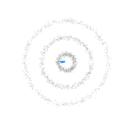
This is terrible though… the middle is almost never where a dart actually lands. The “optimal” guess is a spot that no darts ever land.
This is the core problem of generative modeling. When a prediction has many valid answers, the best single prediction is their average, and the average of data is generally a bad answer that looks nothing like the real data.2
And this problem isn’t special to dartboards or dogs, it shows up with any kind of data. When we trained a model to directly generate three piles of 2D points, it predicted a single dot in the middle of them, and when we trained one on text, all it could say was “the”.
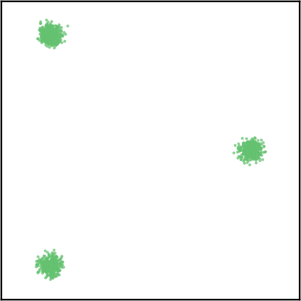
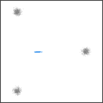
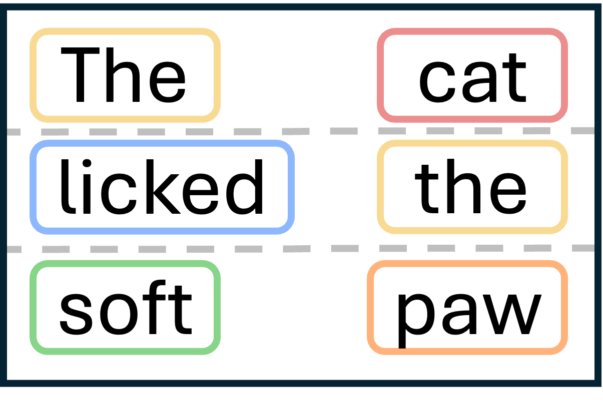
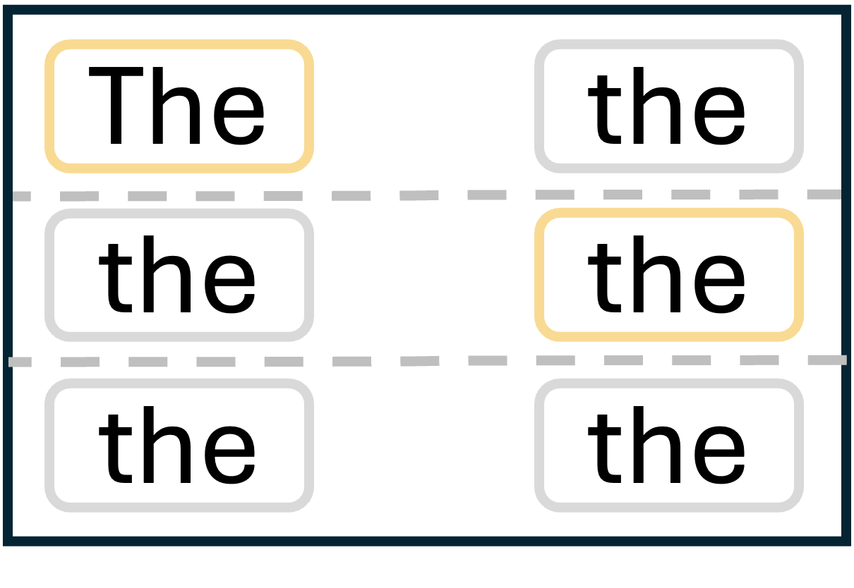
But wait. ChatGPT writes coherent text, and image models generate really amazing images. Clearly this problem has been solved somehow, right?
It has, and every scalable generative model today solves it the same way, by breaking generation into many small steps during training, so each step has roughly one right answer. When a step has one right answer, there’s nothing to average, and the blur disappears.
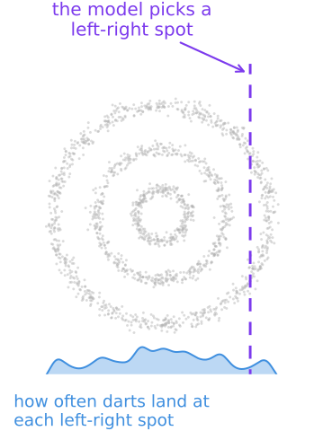
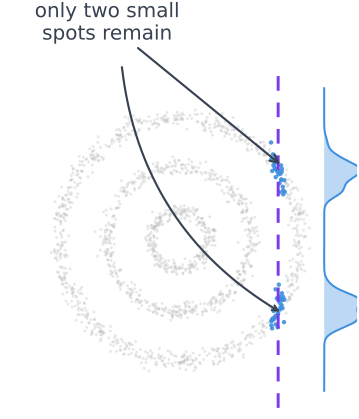
Let’s look at how this works. Autoregressive models (like LLMs) predict one piece at a time, which in our game means never guessing the dart’s exact position all at once. Instead, you first guess only how far left or right the dart lands, and then given that, you guess how far up or down. Once you know the dart landed on the far right, there are only a couple places it could be.
Diffusion models do this differently. They start from pure random noise and take hundreds of tiny steps toward the data. Early on, their guess could still become any dart, but every step narrows the possibilities, so no single step ever faces many valid answers at once.
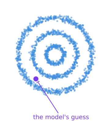
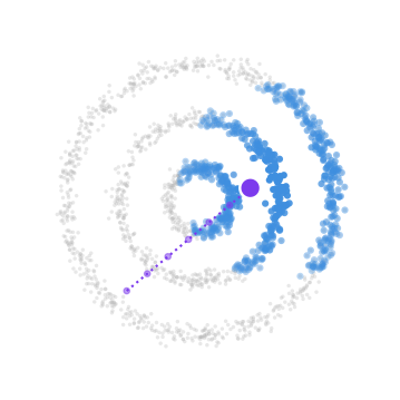
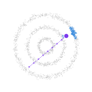
It turns out this is basically how every modern generative model works, by breaking the generation process into smaller pieces that can be predicted well. This includes LLMs, image and video models, and even newer few-step models like MeanFlow and consistency models. We refer to this idea of breaking generation into pieces as factoring generation.
This approach of factoring generation works, but it’s also evil for a couple of reasons. The first is that models get trained on a single step, yet run for hundreds or thousands of steps at inference, so their own imperfect outputs get fed back in as inputs, errors compound, and generations slowly drift away from anything the model saw during training. This problem is called exposure bias (I wrote a whole blog on why it’s evil), and it’s why video models melt into mush after ten seconds and why LLMs get less coherent over really long generations, directly hurting performance and generalization.
The second evil builds on the first, because that mismatch between training and inference means these models are never end-to-end, where an end-to-end model runs at inference exactly the way it was trained. End-to-end learning is what kicked off the deep learning revolution with AlexNet, and the lesson has held ever since… letting models learn everything directly from data beats hand-designing parts of the pipeline, and a model that runs the way it was trained is never forced into out-of-distribution territory. Nearly all of deep learning has gone end-to-end by now except generative modeling, and factoring generation is exactly what’s blocking it.
So ideally we’d stop factoring generation, but factoring is also the only trick we know that handles the many-answers problem. The natural question then is whether we could factor something else instead, and it turns out a generative model only has two processes, how it generates and how it trains. If generation is off the table, that leaves the training loop.
So what does factoring training look like? To answer this, let’s go back to our game, except this time I’ll give you twenty guesses instead of one, and only your closest guess counts. It turns out that with twenty guesses, guessing the middle becomes a terrible strategy. This is because you can now spread your guesses over the spots where darts actually land, lowering your error far more than the middle ever could. In other words, the winning strategy is to use your guesses to explore different answers.
And this is exactly what happens. When we train a model this way with twenty guesses (middle panel below), its guesses spread across the board!
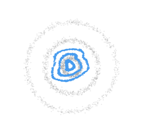
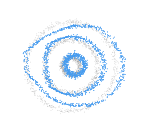

Take a second to appreciate what just happened here. The darts land in the exact same places as before, but because we changed how guesses are scored, the best possible prediction moved from the middle of the board onto the spots darts actually land. This reveals something important, which is that the training objective alone controls what the best prediction is (the loss minimizer), and by changing it, we moved the loss minimizer from the average of the data onto the data itself.
This is Explorative Modeling. At each training step, the model explores K possible matches between what it generates and the real data, and only the best match gets trained. We call models trained this way Explorative Models (XMs). In the simplest case, this is literally, beautifully, a for loop:
losses = []
for i in range(K):
    generation = model.generate()  # e.g., from a different random noise
    losses.append(loss_fn(generation, data))
min(losses).backward()  # only the best generation gets gradients
Here’s what happens as we increase the exploration K on real data:
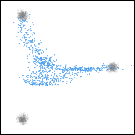
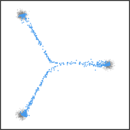
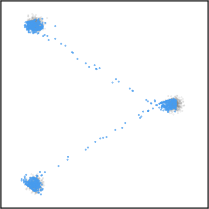
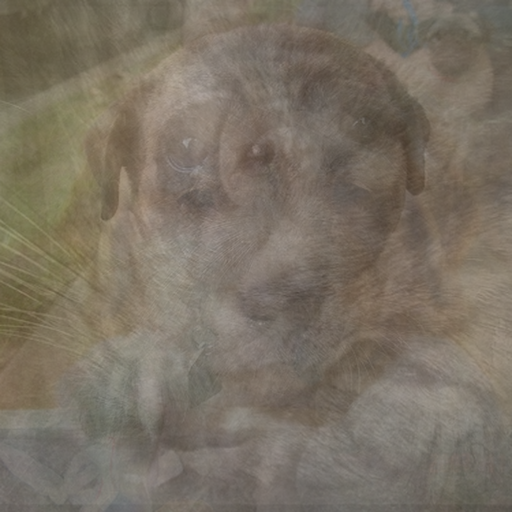


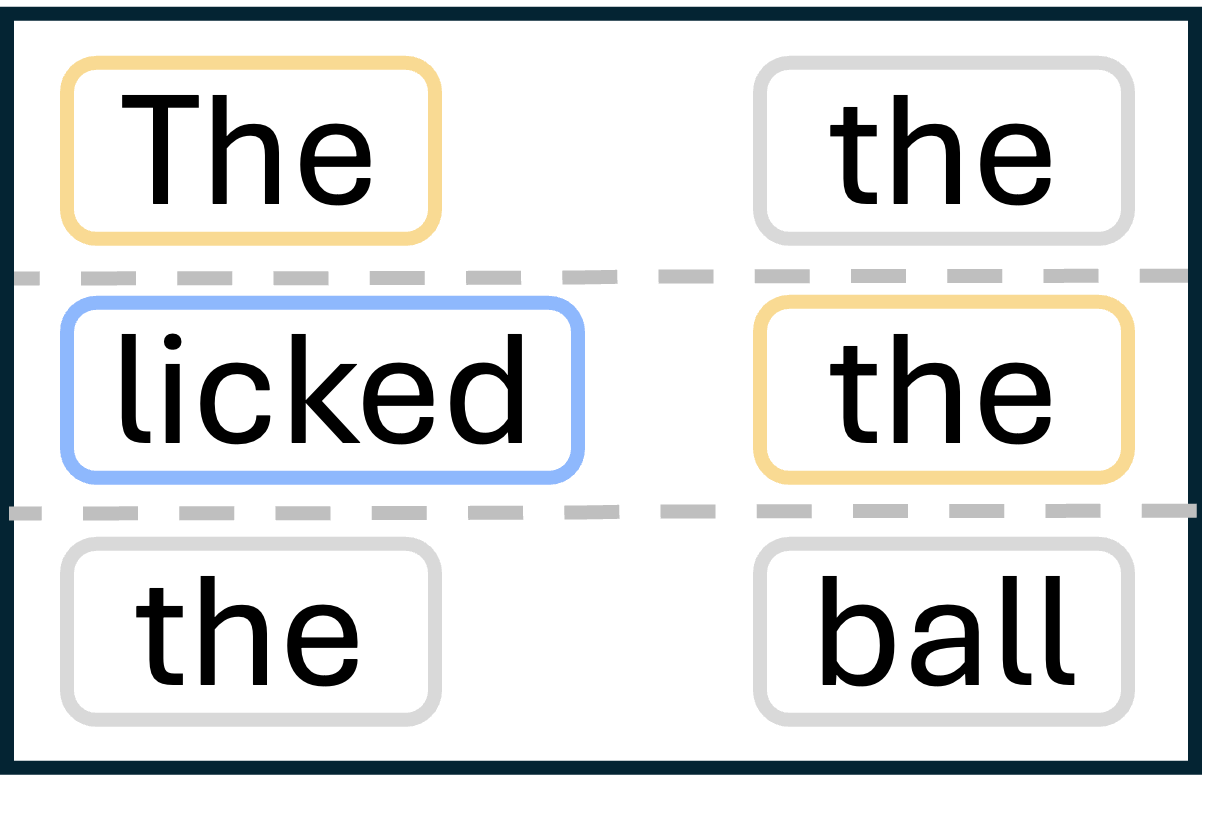
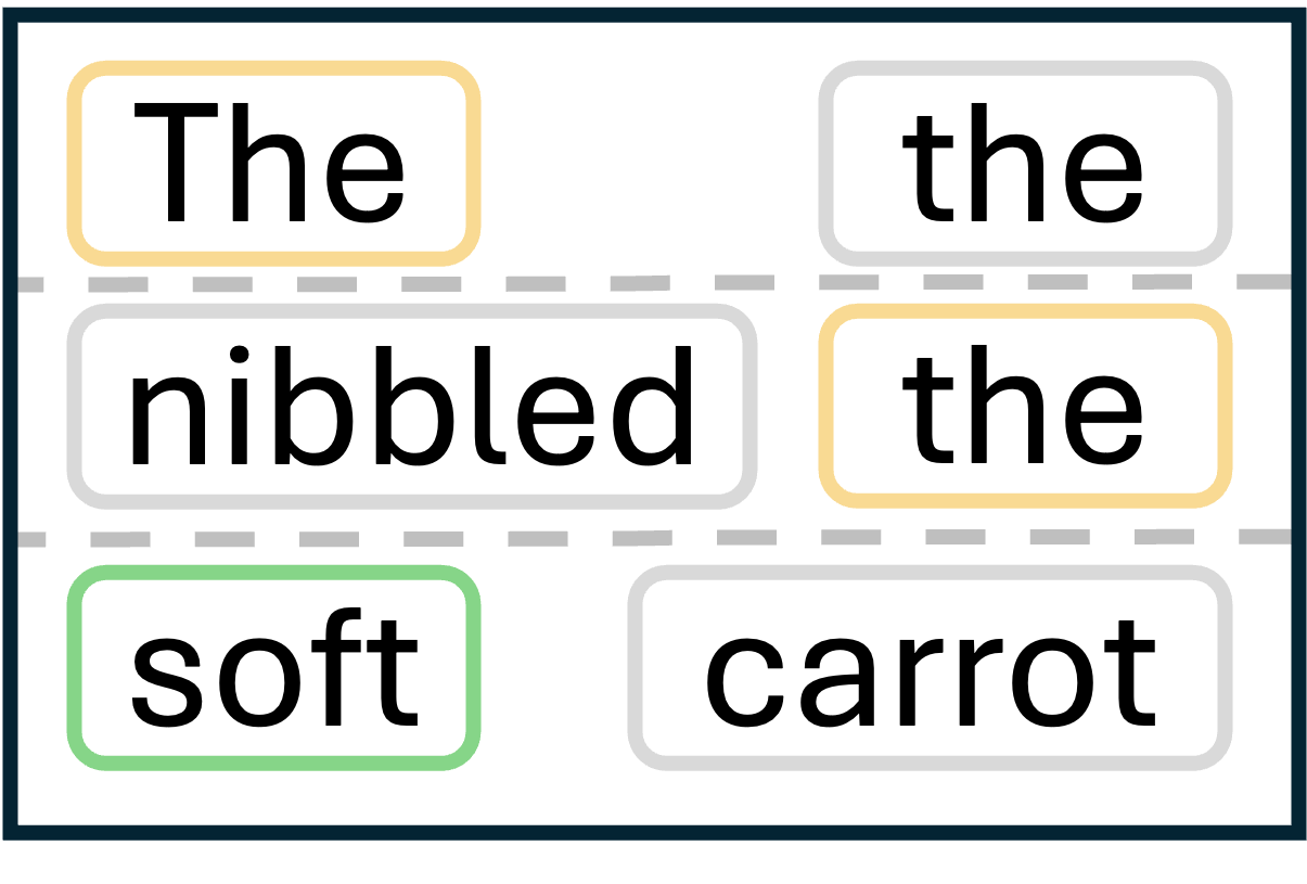
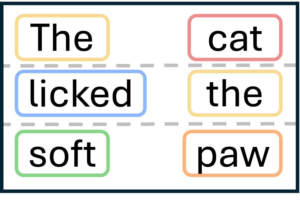
If we zoom out, this figure actually hints at something much bigger. All of modern generative modeling is really about designing a training objective whose loss minimizer lands on real data instead of between it, and factoring generation and exploration are just two different ways of achieving this. We call this idea Mode Forcing, and it’s the theory that led us to Explorative Modeling in the first place, predicting almost every result in the paper before we ran the experiments. There’s a whole paper on Mode Forcing coming soon :)
Another thing worth noticing is that all of an XM’s extra work happens during training. For end-to-end XMs, generation itself is left completely untouched, staying a single step that works identically during training and inference.
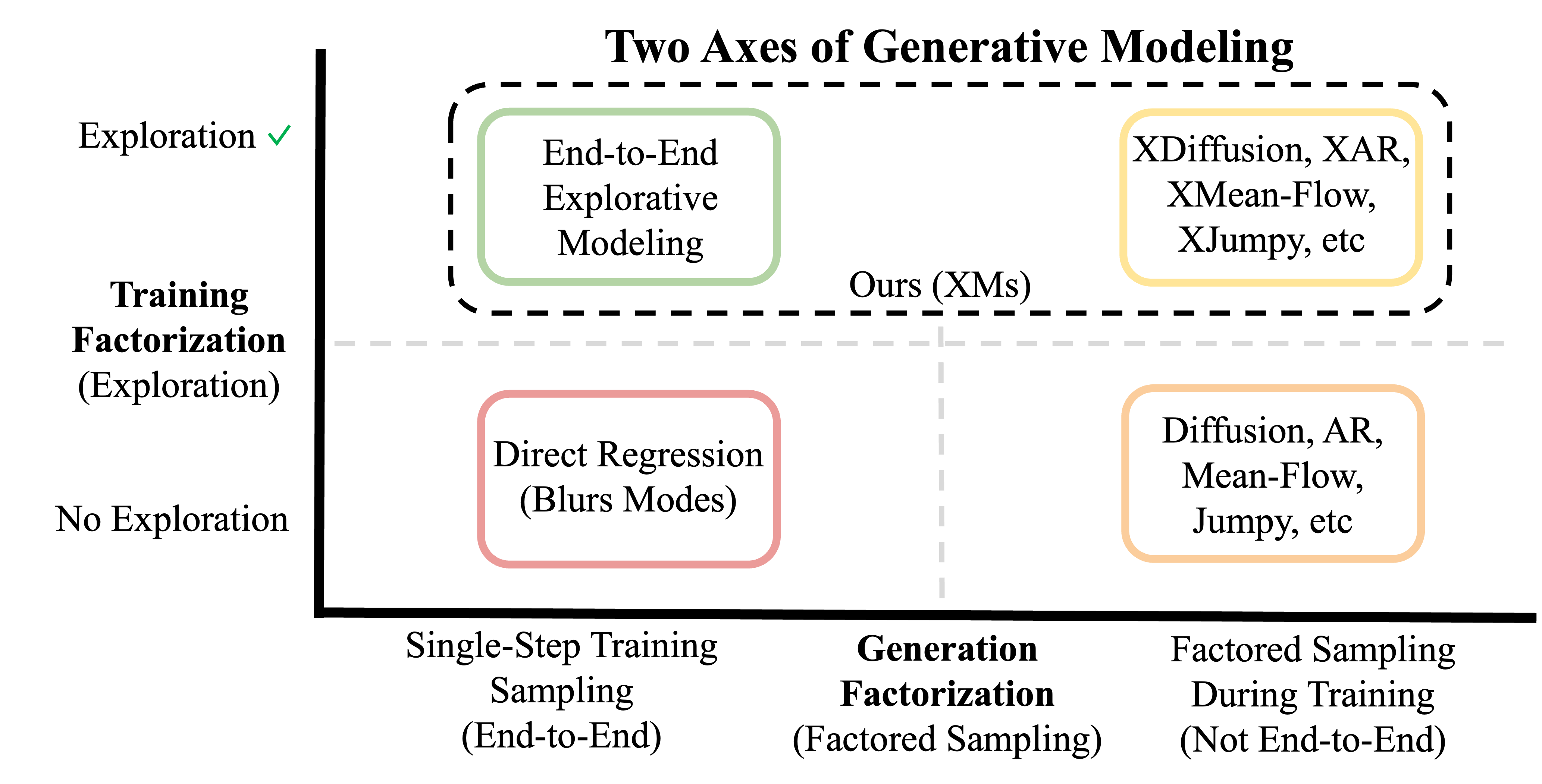
So why does exploring more keep helping? It turns out that K controls how many distinct answers a model can commit to. With one guess, the model has to average everything, but with twenty, it can commit to twenty different answers that each specialize to a different part of the data. In the paper we call this capacity generative expressivity, the number of distinct answers a model can capture.
What’s crazy is that generative expressivity has been almost completely overlooked, to the point where the term didn’t even exist before this and the Mode Forcing paper.3 Yet it matters just as much as parameters and data. A model with a single parameter can’t do much no matter how much data you feed it, and in the exact same way, a model with a generative expressivity of one can’t do much no matter how many parameters and data you give it… its best possible output is still the blur (look at the K=1 column of Figure 8). For over a decade we’ve scaled parameters, which set what a model can represent, and data, which sets what a model can learn, while generative expressivity, what a model can generate, has stayed fixed, baked into the training objective. Factoring generation was the field’s fix for this, but the expressivity it supplies is frozen the moment you design the model, whereas exploration turns it into something you can actually scale. This is exactly why scaling generative expressivity through exploration is a third pretraining axis, and as we’ll see below, the empirical results back this up.
At this point we know what Explorative Modeling is, so how do we actually use it? Looking back at Figure 9, there are two ways, combining exploration with existing generative models, or using it as a standalone approach. Combining exploration with existing models is where the new pretraining axis comes from, whereas using XMs as a standalone approach is what enables end-to-end generation.
Let’s start with existing generative models. At first glance it might seem like they don’t need more generative expressivity, since factoring generation already handles the many-answers problem. But if you look closely, single steps inside diffusion or autoregression can still face many valid answers at once, meaning some blurring remains.4 Even worse, as models and datasets grow, parameters and data stop being the bottleneck while generative expressivity stays frozen, so we’d expect it to increasingly become the thing holding models back. If all of this is true, then adding exploration to existing models should improve them, with gains that grow with scale.
To test this, we added exploration on top of existing generative models while changing nothing else about their recipes, not even the hyperparameters.
We started with RAE, the ~state-of-the-art ImageNet generation recipe. Adding exploration reaches RAE’s final performance with 6.2× less data and 4.1× fewer FLOPs, and hits a ~state-of-the-art 1.43 FID on ImageNet 256 without guidance. The speedups also compound across recipes, where XRAE converges 6.2× faster than RAE, which itself converges 47× faster than the standard SiT recipe, making XRAE almost 300× faster to converge than SiT.
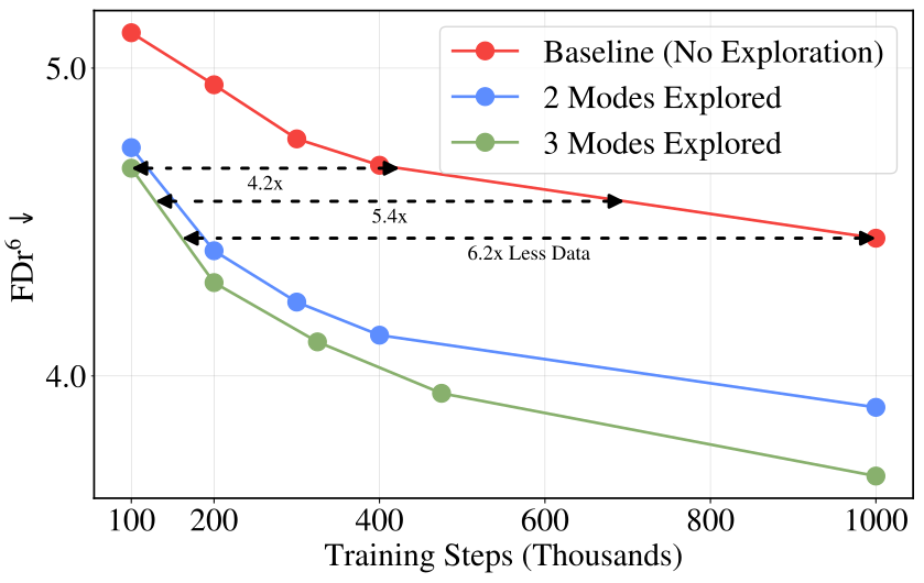
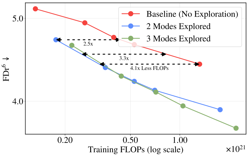
The same story holds on an optimally tuned SiT baseline trained at a third of the compute, where exploration improves FLOP efficiency by up to 52% and reaches the same performance with 2.5× less data.
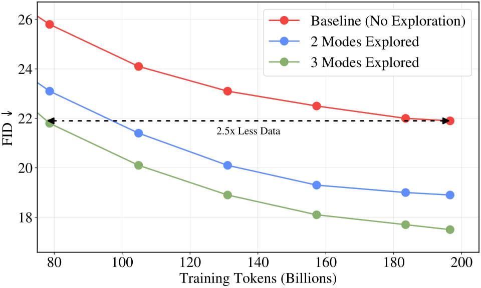
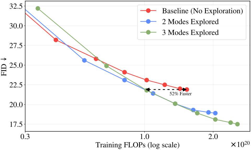
There’s also a subtle hint hiding in these plots, where the compute-optimal amount of exploration grows over the course of training (look at the crossovers in the FLOPs plots), directly mimicking how the compute-optimal number of parameters grows with compute in Chinchilla scaling. This reinforces that exploration really is a new pretraining axis, along with some more results below.
We also tested this on domains beyond images, adding exploration to video generation and masked diffusion language models while varying only the amount of exploration. In every domain, more exploration steadily improved performance, with some video models gaining over 20%, and the gains showed no sign of stopping at the largest K we tested.
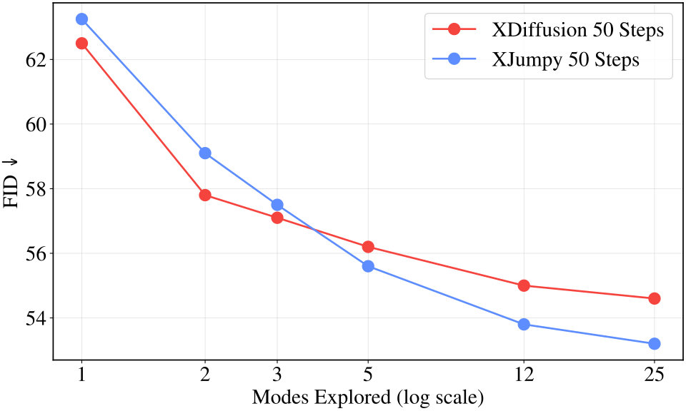
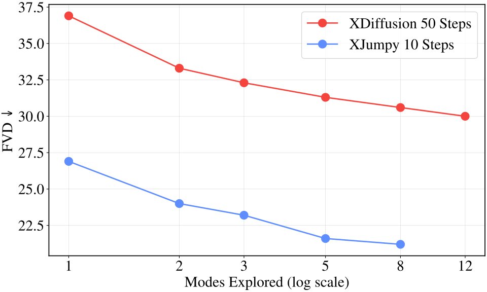
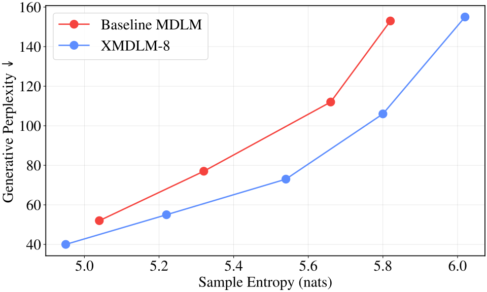
The most important result, though, is that the gains from exploration grow with scale. As data scaled, gains rose from 7% to 36%. As models scaled, gains rose from 13% to 23%. And the efficiency gains above more than doubled when we tripled the compute. This is exactly what you’d expect if generative expressivity is a real third axis. Small models are held back by parameters and data, but as those scale, the fixed generative expressivity increasingly becomes the bottleneck, and exploration is what relieves it.
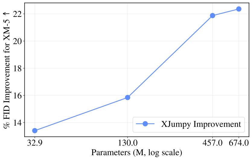
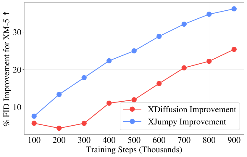
For reference, frontier training runs use roughly 10,000× more compute than our largest experiments. If these trends of gains growing with scale hold, the numbers here are probably a lower bound.
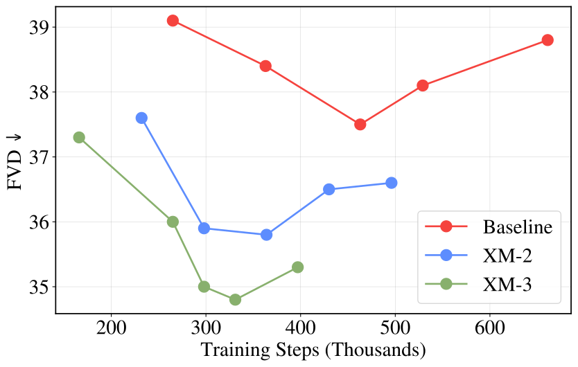
It turns out exploration improves generalization as well. To see why, remember that during pretraining the same input often gets paired with many different valid targets, which to a model that can only predict one thing looks like noise, and fitting noise is memorization. With exploration, each prediction instead trains toward the target it’s already closest to, so the targets become consistent and what looked like noise becomes structure the model can actually learn.5 We see this directly in our experiments, where models with more exploration overfit less on a fixed dataset and reach better performance (a best FVD of 30.0 vs 37.5 without exploration). In other words, extra training compute directly buys generalization, which I find especially exciting as data, not compute, increasingly becomes the bottleneck for large-scale training.
So exploration clearly works as a pretraining axis, but what about end-to-end generation? One of the biggest implications of generative expressivity is that factoring generation and exploration supply the exact same thing, which means they should be interchangeable. We demonstrate this directly below, where as exploration increases, the best-performing models use less and less generation factorization, meaning models that are more end-to-end benefit the most from exploration.
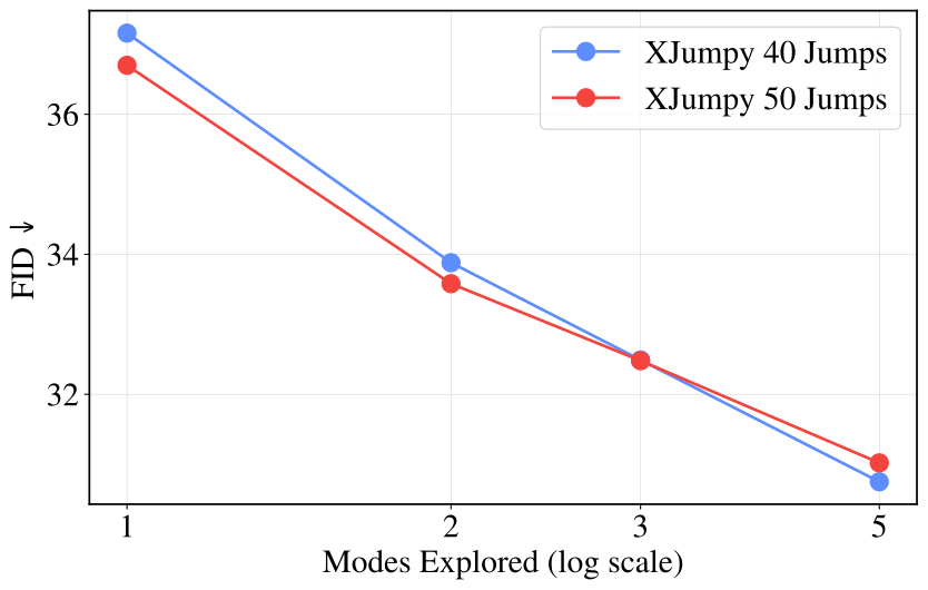
This makes how end-to-end your model is not a fixed design choice, but rather something you can scale. We can scale end-to-endedness :)
Taking this to its limit, we trained fully end-to-end XMs, where sampling is exactly the same at training and inference. On behavior cloning, our Explorative Policy matches Diffusion Policy with a single forward pass instead of 100:
| Method | Forward passes | Lift | Can | Square | Transport | Tool Hang |
|---|---|---|---|---|---|---|
| Diffusion Policy | 100 | 100% | 100% | 94% | 72% | 86% |
| Explorative Policy | 1 | 100% | 100% | 96% | 74% | 86% |
And our Explorative World Model matches Diffuser on goal-conditioned world modeling with 16-256× fewer forward passes:
| Method | Score (avg) | Forward passes (avg) |
|---|---|---|
| Diffuser | 127.2 | 192 |
| Explorative World Model | 130.0 | 2.3 |
The reason this is even possible comes back to what each approach factors, where diffusion pays for its generative expressivity with generation steps at inference, while XMs pay for it through exploration during training.
So where does this leave us? If you train robotics policies, world models, image, video, or audio generation models, masked diffusion language models, or really any generative model whose predictions face many valid answers (i.e., models working on decently multimodal distributions), you can add exploration with a for loop, without touching your architecture or hyperparameters (there’s pseudocode on the website if you want to try). In our experiments, adding exploration improved FLOP efficiency, data efficiency, parameter efficiency, and generalization across every domain we tried, so there’s a good chance it does the same for you! The best way to predict whether XMs will help is to determine how many valid answers each of your model’s predictions faces. The more answers per prediction, and the bigger your scale, the more exploration has to offer, while predictions with one clear answer (less multimodal) will likely benefit less (although benefits are still possible, as the paper discusses and lightly experiments with).
This rule of thumb also explains why autoregressive LLMs are the one place we’ve tested so far where exploration hasn’t been an immediate win, since predicting the next token given a long context is already close to having one right answer, and LLMs have no natural latent variable to explore over. That said, we’ve already seen modest early gains in data efficiency for autoregressive LLMs, and we have several ideas for pushing further, such as multi-token prediction, which faces far more valid answers per prediction, or conditioning on a learned latent, which would give exploration something to search over. I believe exploration will eventually make LLMs more end-to-end and better-scaling too, it just needs more work.
Longer term, the two directions I’m most excited about are Reverse XM and gradient-based exploration. Reverse XM flips the search so that one generation searches over K datapoints instead of one datapoint searching over K generations, which costs almost no extra compute and in principle lets K grow to the size of the entire dataset. Gradient-based exploration would replace random guessing with directly descending the loss to find the best latent. Pushed far enough, either one turns generative modeling into pure search for good latents with a very large K.
Taking a step back, the coolest part of this project to me is where it all came from. It didn’t start with tinkering or a lucky ablation, it started with deeply understanding why generative modeling is hard, which to me was an aha moment that resulted in all of Mode Forcing and ultimately ended up resulting in predicting all these results beforehand. And if you look back, that’s exactly the path this blog just walked… we started from first principles, arrived at Explorative Modeling as a way to increase generative expressivity, and from there got both a new pretraining axis and end-to-end generation.
If there was one takeaway from this paper, I’d say it’s the following:
We scale the size of generative models and how much data we train them on… so why haven’t we scaled what they can generate?
Huge thanks to my collaborators Yilun Du and Heng Ji, and to everyone who supported this work! Check out the paper and website for more details/depth!
Citation
@misc{gladstone2026explorativemodelingunlockingpretraining,
      title={Explorative Modeling: Unlocking a Third Pretraining Axis and End-to-End Generation},
      author={Alexi Gladstone and Heng Ji and Yilun Du},
      year={2026},
      eprint={2607.27372},
      archivePrefix={arXiv},
      primaryClass={cs.LG},
      url={https://arxiv.org/abs/2607.27372},
}
Footnotes
-
Being scored by squared distance means your best guess is the average of all landing spots, and for rings centered on the board, that average is the exact middle. ↩
-
The formal name for this is a multimodal distribution, a distribution with many distinct peaks (called modes), where each mode is a valid answer. The paper talks about “capturing modes instead of averaging them”, which is this exact idea. ↩
-
To be fair, people have long known that generative models need to capture modes instead of averaging them, and problems like mode collapse are well studied. What’s been missing is formalizing this as a capacity of the training objective itself, and recognizing just how central it is. Mode Forcing’s core claim is that having enough generative expressivity is the most important property of a generative training objective, and that even modern approaches like diffusion and autoregression have a fixed amount of it, a fundamental limit that scaling parameters and data can’t fix. ↩
-
There’s fun indirect evidence for this. Classifier-free guidance, which nearly all image models rely on, improves samples by pushing them away from a blurrier version of the model. If models weren’t blurring at all, there would be nothing to push away from. ↩
-
This is similar to overparametrization, where models with more parameters than they strictly need generalize better because the surplus capacity makes good solutions easier to find. Surplus exploration seems to do the same thing for generation. ↩
Enjoy Reading This Article?
Here are some more articles you might like to read next: